El Farol with local imitation on a grid
Project for "Controversies in Game Theory" by Lukas Münzel, Pascal Gamma, and Nandor Kovacs
Introduction
Inspired by the paper on cooperation and defection on a grid that was presented in class1, we decided to study El Farol with players on a grid all going to one bar but only locally exchanging information.
The broad approach of studying El Farol with players imitating strategies of neighbors is admittedly not novel23456. However, this existing literature does not seem to have discouraged previous authors from studying their favored setup. Given that the specifics of our setup were entirely developed by us before we were aware of any similar studies, it seems highly unlikely that the exact setup we study already exists.
Furthermore, all existing literature we stumbled on in three hours of literature search does in fact differ from our setup in some way. For example, in Kalinowski et al.2 the players know the previous decisions of their neighbors, whereas in our setup they are only aware of the previous attendance rates, Slanina3 uses imitator and leader roles with imitation being costly, and Chen et al. 6 play on a random graph instead of a grid. We therefore feel that our work is not entirely derivative and hope it will be of interest to the reader.
Preliminaries
Nash equilibria of El Farol
A simple strategy is to go to the bar with probability \(0.6\) and stay at home with probability \(0.4\). If all players use this strategy, none can improve their payoff by changing to a different strategy7. Therefore, this strategy is a symmetric (non-cooperative) Nash equilibrium.
Furthermore, if 60% of the players always go while the rest always stay at home, there is no way for a single player to increase his expected payoff and thus this is a Nash equilibrium as well. Such Nash equilibria are called corner solutions7.
Optimal strategy given fixed opponents
Nearly all strategies we handcraft for El Farol in one way or another estimate the anticipated occupancy of the bar and go to the bar if and only if this expected occupancy is less than 60 percent. These strategies always return the mean occupancy in expectation. This is also the case for most strategies proposed in the original El Farol paper8 by Brian Arthur.
But is this actually optimal? Suppose we are dropped into an environment in which all other actors engage a strategy that is potentially random but does not depend on previous occupancy rates. So let \(X\) be the random variable representing the percentage of other players attending. Then it is in fact in general not optimal to the “anticipated occupancy” to be the mean of \(X\).
Indeed, the expected return of a strategy is given by
\[\begin{align*} P(\text{going},\text{bar is not full}) + P(\text{not going},\text{bar is full}) &=P(\text{going})P(\text{bar is not full}\;|\;\text{going}) + P(\text{not going})P(\text{bar is full}\;|\;\text{not going}) \\ &\approx P(\text{going})P(X < 0.6) + P(\text{not going})P(X > 0.6) \end{align*}\]Note that this is only approximate because there is some small chance that our decision to go is actually what shifts the bar from not being full to being full.
This approximation yields another result of interest to us: When \(P(\text{X > 0.6})=0.5\), all strategies give basically identical payoff in expectation. Thus, if, say, all other players are playing the Nash equilibrium, all possible strategies for the remaining player are equivalent.
Simulations
Setup
We simulate multiple iterations of the El Farol bar game on a two-dimensional grid of side length \(n\) with \(n^2\) players and one bar. Every iteration consists of five rounds of El Farol in which each player decides whether or not to go to the bar based on the attendance rates in previous rounds. Like in the original paper8, we consider the bar crowded if more than \(60\%\) of the players choose to attend. We use a symmetric payoff: a player’s action is considered a success if they go to the bar when it is not crowded or stay at home when it is crowded. Each player receives a payoff of \(1\) for each successful and \(0\) for each unsuccessful round.
After the end of an iteration, each player may choose to adopt a strategy of one of his neighbors based on its performance over the last five rounds.
Handcrafted strategies with discrete updates
Methods
First, each player chooses uniformly at random from a list strategies similar to those proposed in the original paper8. At the end of each iteration, each player chooses to imitate a strategy in their Von Neumann neighbourhood.
More specifically, we play on a grid of size \(100 \times 100\) with up to \(16\) distinct strategies. In each iteration, every player decides based on their current strategy whether to attend the bar or stay at home. The attendance rate is computed and the players get rewarded according to the symmetric payoff as described. Then each player’s strategy is updated based on the following procedure:
Let \(P_0\) be the current player and \(P_1, \dots, P_4\) the neighbors with scores \(S_0, \dots, S_4\) respectively. With probability \(R\), which we will call the retention rate, the player retains their current strategy. Otherwise they adapt to the strategy of player \(P_i\) with probability \(\frac{\exp(S_i/T)}{\sum_{j=0}^4 \exp(S_j/T)}\) where \(T > 0\) is called the temperature. Notice that as \(T\) approaches \(0\), this softmax converges to the argmax and as \(T\) approaches infinity, it converges to a uniform distribution. We therefore by slight abuse of notation denote the argmax as \(T=0\).
Results and Discussion
Observe first that if we set both the retention rate \(R\) and the temperature \(T\) to zero, the game is deterministic and entirely determined by the initial configuration. In this case the players always adapt to the best strategy in their neighborhood.
We randomly initialize the grid with two simple strategies: always go and always stay at home. In the first iteration, roughly half of the players go to the bar and the bar is therefore not crowded. Thus, the always go strategy receives higher payoff and, consequently, any player that has at least one neighbor using this strategy adopts it. There then are too many players attending the bar in the next iteration, making it crowded. However, because the players only look at their immediate neighborhood while adapting their strategies, there are some always stay home players left that happened to be completely surrounded by others with this strategy. Here, we see the advantage of only considering other strategies in a small neighborhood. Indeed, if we considered the best strategies in a larger radius, the always stay home strategy would completely die out and all players would be worse off.
In our setup, we instead observe pulsating behavior: The bar is overcrowded in one iteration and under-attended in the next one because too many players adapt to what would have been the best strategy in the previous round. This overshooting is the reason why we don’t observe convergence to the corner solution.

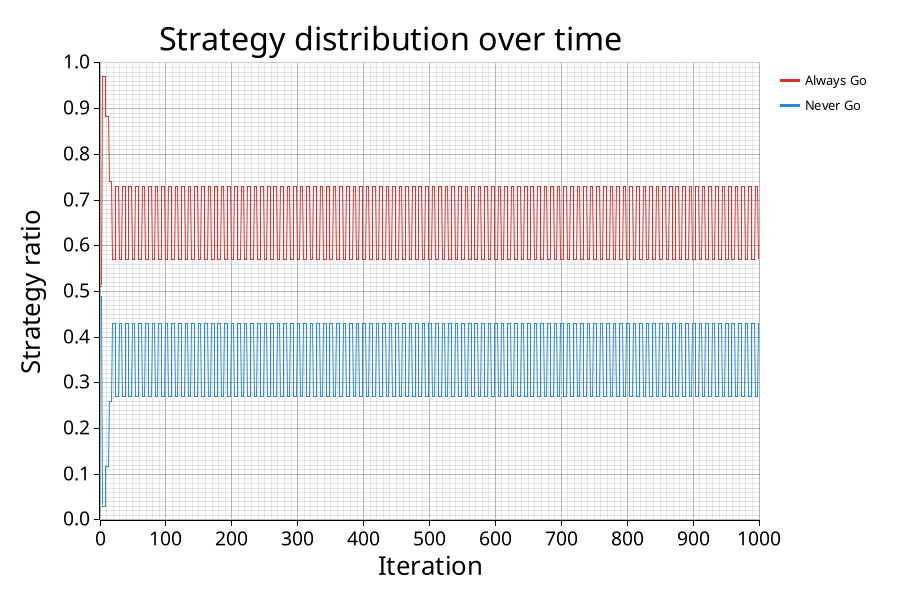
Two simple strategies are enough for the attendance rate to stay around 60%. (T=0.0, R=0.0)
When we introduce more strategies, an interesting phenomenon emerges: The random strategy dominates and eventually all players adapt to it. This appears to be happening because the random strategy is the only strategy that is robust to its own popularity: it performs the same way regardless of how many players adapt to it. On the other hand, most other strategies tend to suffer from their own success: When many players follow the same deterministic rule, the bar is always occupied far above or below its \(60%\) capacity.


The random strategy outperforms all the others. (T=0.0, R=0.0)
Removing the random strategy results in an equilibrium of multiple strategies coexisting. Interestingly, the specific set of surviving strategies is not fixed and depends on the initial configuration. As long as the strategies are sufficiently uncorrelated, they can coexist with the same kind of pulsating behavior as seen in the simple case above. However, the dynamics are a lot more complex because of the number of strategies at play. In fact, we occasionally see some tipping points where suddenly the ratio of the strategies changes significantly from one iteration to the next. This can be explained by the dependence of many strategies on the average attendance rate of all previous rounds. This number changes continuously over time but as soon as it hits a certain threshold (e.g., \(60\%\) for the simple case of the full history average strategy) the behavior of the agents and consequently their performance changes immediately.


Multiple strategies coexist when the random strategy is not present. (T=0.0, R=0.0)
As the retention rate and temperature are increased, players no longer immediately adapt to the best strategy in their neighborhood. With \(R=0.9\), the players only update their strategy, on average, after \(10\) iterations. The higher temperature leads to the players sometimes also adapting to a strategy that did not strictly perform best. This leads to less overshooting, which is why we observe far less fluctuation both in terms of both the attendance rates and the frequency with which which strategy is played.


Smoother convergence with higher retention rate and temperature randomness. (T=1.0 and R=0.9, no random strategy)
Even though we have much more stable behaviour with \(T=1.0\) and \(R=0.9\), the random strategy dominates when it is present. That this happens after around \(\approx1800\) instead of the previous \(\\approx 250\) iterations can be attributed to the decelerating effect of a higher retention rate. This convergence to the symmetric Nash equilibrium appears to be a remarkably robust phenomenon: Even small variations in different parameters or minor modifications to the update mechanism consistently led to this behavior over multiple runs.


The random strategy still dominates. (T=1.0, R=0.9)
Random strategies with “gradient descent” updates
Methods
We now investigate continuously parametrized strategies that update via “gradients” instead of outright copying successful strategies. More concretely, at the beginning of each iteration, each player \(k\) has some parameter \(p_k \in [0,1]\). In each round of that iteration, the player will go to the bar with probability \(p_k\) (naturally, sampled independently of the round and the player).
After all rounds of the iteration have been played, the players count and compare their successes (a success being defined as going to the bar when it is less than \(60\%\) full or vice-versa not going when it is). We choose the player \(l\) from the four neighbors in the Von Neumann neighbourhood of \(k\) with the highest number of successes (or any maximal neighbor should this not be unique). Then we update \(p_k\) by increasing it by some \(\delta > 0\) if \(p_l>p_k\) or, if \(p_l < p_k\), decreasing it by \(\delta\)
In our tests for this section, we also add periodic boundary conditions in the sense that we map the grid to a torus. So, for example, the top left cell has the bottom left or the top right cell as neighbours. This has the advantage that if \(p_1, \cdots, p_n\) are initially sampled i.i.d. from some distribution \(\mathcal D\) on \([0,1]\), \(p_1, \cdots, p_n\) are identically distributed even after the updates described above.
We also compare against a strategy where every player takes a step of size \(\delta\) towards what the optimal strategy would be if all other players would not modify their strategy. Concretely, we estimate the median attendance given the current distribution of \(p_k\) and increase \(p_k\) by a \(\delta'\) chosen uniformly between \(0\) and \(2\delta\) if it is smaller than \(0.6\). The reason why we don’t just move all players by \(\delta\) is that we could essentially not decrease variance as we just shift the entire distribution.
Results and Discussion
We first take \(\mathcal D\) to be the distribution assigning probability \(0.5\) to \(0.25\) and \(0.95\). With updates local updates (i.e. updating towards the best strategy in the Von Neumann neighborhood) and a grid length of \(128\), we get the following result:
We can observe that we get some combination of diffusion with some sort of convergence to the Nash equilibrium given by \(p=0.6\).
We also include a plot the entropy of the distribution of the \(p_k\) over time for different values of \(\delta\):
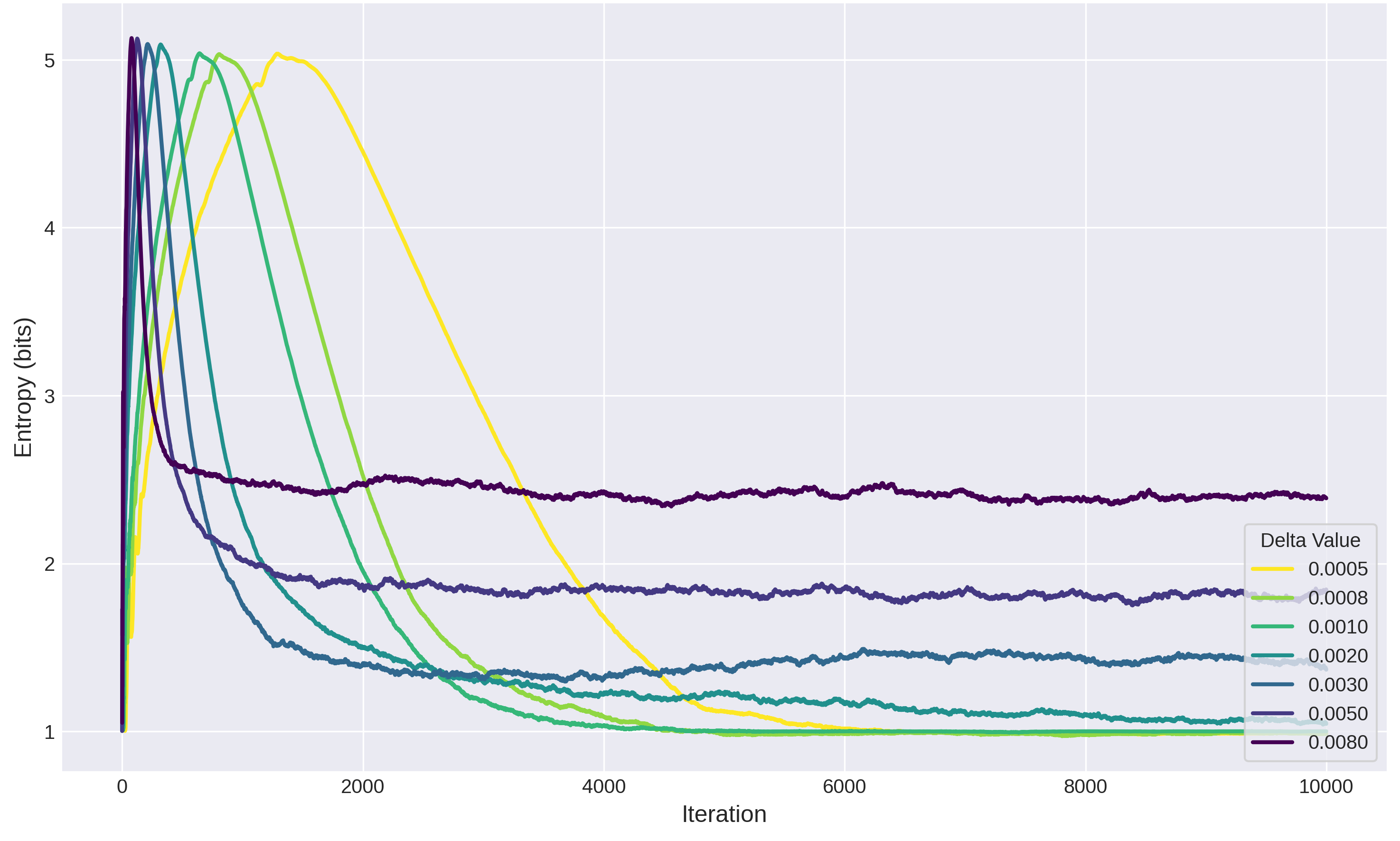
Evolution of entropy for various values of delta
One can observe an initial increase in entropy as the probability mass diffuses away from \(0.25\) and \(0.95\) followed by a decrease as it starts concentrating more and more around \(0.6\). Also note that, as one might expect, this transition occurs faster the higher the “learning rate” \(\delta\) is.
We see that we get some form of convergence to the Nash equilibrium when doing local updates but no convergence at all in the case where we do the updates that are globally optimal:
Time evolution of distribution for p initially having only two values as described before.
Local updates are to the left, global updates to the right
Time evolution of distribution for p initially having uniform distribution.
Local updates are to the left, global updates to the right
In fact, this does make sense. When only doing globally optimal updates with some noise, we shift until the median occupation hovers around \(60\%\). But after that, there is no more drift distribution of \(p_k\) when doing globally optimal updates because all strategies are equivalent, as was elaborated in a previous paragraph.
On the other hand, when doing local updates, there is a bias towards the mean because there is noise in evaluating neighbor has the best strategy and thus there is some bias towards the mean of the neighbors. This biases the time-evolution of the distribution towards its mean and thus a bias towards \(0.6\).
We also quickly verify that the mean p does in fact eventually hover around \(0.6\) even when the initial distribution is uniform:
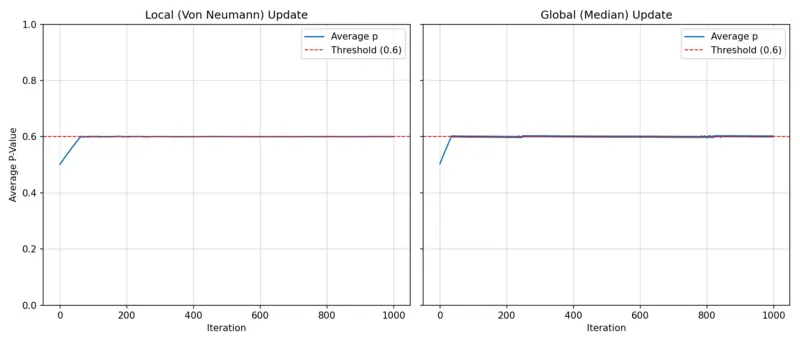
Average attendance over time with local and global update rule
Again, this makes sense: When, for example, the median attendance is below \(0.6\), we get a net increase of the mean \(p\) as neighbours with higher \(p\) on average perform better. In the global case, the picture is even clearer because we increase all \(p_k\) if the median attendance is below \(0.6\).
Conclusion
The simulations with the handcrafted strategies and discrete updates demonstrate the advantage of local over global information exchange and updates. Restricting players to only observe strategies in their immediate neighborhood helps to preserve a more diverse set of strategies, which in turn helps to keep the attendance rate closer to \(60\%\).
Most notably, we observe that the random strategy dominates across the vast majority of parameter settings. Unlike deterministic strategies, which tend to perform worse as they become more widely adopted, the random strategy performs consistently regardless of its popularity. It is able to spread to the whole population resulting in our setup consistently converging to the Nash equilibrium.
Interestingly, we observe the exact same behaviour when analyzing the continuously parametrized strategies with gradient updates: Trying to make decisions based on global information results in unstable, non-convergent behaviour while updating only based on what seems optimal locally results in convergence to the Nash equilibrium.
Appendix
Explanation of the handcrafted strategies
Let \(b_i\) be the attendance ratio \(i\) rounds ago.
| Name | Explanation |
|---|---|
| Always Go | Always goes to the bar. |
| Never Go | Never goes to the bar. |
| Predict from yesterday | Goes to the bar if less than \(60\%\) were there in the last round. |
| Predict from day before yesterday | Goes to the bar if less than \(60\%\) were there two rounds ago. |
| Random | Goes if a uniformly generated random number between \([0, 1]\) is less than \(0.6\). Note that this is the same as \(\operatorname{Ber}(0.6)\). |
| Moving Average (\(m\)) | Goes if the average attendance of the last \(m\) rounds was less than \(60\%\). |
| Full History Average | Goes if the average attendance was less than \(60\%\). |
| Even History Average | Goes if the average of the even rounds was less than \(60\%\). |
| Complex Formula | Goes if \(\frac{1}{2} \left[ \sqrt{\frac{1}{2}(b_n^2 + b_{n-1}^2)} + b_{n-2} \right]\) is less than \(60\%\). |
| Drunkard | Goes if the average attendance was less than \(65\%\), because he really likes to go to the bar. |
| Stupid Nerd | Goes if the average attendance was less than \(55\%\), because he does not really like to go to the bar. |
| Generalized Mean | Goes if \(\left( \frac{1}{m} \sum_{i=1}^m b_i^r \right)^{\frac{1}{r}}\) is less than \(60\%\). Notice that in the case of \(r=1\) this is just the arithmetic mean, \(r=2\) is the root mean square and \(r=-1\) is the harmonic mean. |
In the initial rounds when strategies require historical attendance data that is not yet available, players temporarily change to the random strategy.
Academic integrity statement on responsible use of AI:
- We extensively used code generation tools such as cursor and claude code. All code used to generate the results in this report was proofread by us to a sufficient degree that we are reasonably comfortable being held accountable for any bugs that may be present in it.
- No single word of writing was copy-pasted from Generative AI output. However, such tools were used to get feedback, brainstorm, find grammatical or orthographic mistakes or suggest better formulations while never e.g. ad verbatim copying a phrase.
Signed,
Lukas F. Münzel, Pascal E. Gamma, Nandor Kovacs
Links to code
- Handcrafted strategies with discrete updates, also includes more experiments where random strategy dominates
- Random strategies with “gradient descent” updates
Small remark on time-evolution of distribution
One can observe that we do not appear to actually get honest to god convergence to the Nash equilibrium in the videos showing the time-evolution of the distribution of \(p_k\). Rather, we seem to get stuck after some relatively narrow peak develops. We attribute this to our taking discrete, relatively big steps (\(\delta \approx 0.003\)) which at some point prevent us from getting even closer to \(p=0.6\).
Bibliography
-
Helbing D, Szolnoki A, Perc M, Szabó G. (2010). Evolutionary Establishment of Moral and Double Moral Standards through Spatial Interactions. ↩
-
Kalinowski, Thomas & Schulz, Hans-Jörg & Briese, Michael. (2000). Cooperation in the Minority Game with local information. ↩ ↩2
-
Slanina, František. (2000). Social organization in the Minority Game model. ↩ ↩2
-
E. Burgos, Horacio Ceva, R.P.J. Perazzo. (2002). The evolutionary minority game with local coordination. ↩
-
Shang, Lihui & Wang, Xiao. (2006). A modified evolutionary minority game with local imitation. ↩
-
Jiale Chen, Hongjun Quan. (2009). Effect of imitation in evolutionary minority game on small-world networks. ↩ ↩2
-
Reiner Franke. (2003). Reinforcement learning in the El Farol model. ↩ ↩2
-
W. Brian Arthur. (1994). Inductive Reasoning and Bounded Rationality. ↩ ↩2 ↩3