There is a parameter in Schulmann’s KL divergence estimator which can be chosen arbitrarily. Schulmann simply choses it to be 1, arguing that this yields an unbiased estimator that is always non-negative.

But setting this parameter to one actually give us another very interesting property! Namely, it minimizes the variance of the estimator - at least if the two distributions whose KL divergence we are estimating are close

A quick recall

Defining \(r(x) = \frac{q(x)}{p(x)}\), we observe that \(D_{KL}(P \parallel Q)= \int \log \frac{p(x)}{q(x)} p(x) dx = \mathbb E_p[\log \frac{1}{r}] = \mathbb E_p[-\log r]\), so \(-\log r\) is an unbiased estimator of the KL-divergence.

Note also that \(\mathbb E_p [r] = \int \frac{q(x)}{p(x)}p(x)dx = 1\), and thus \(r-1\) has mean zero.

This implies that for every \(\lambda \in \mathbb R\), \(-\log r + \lambda (r-1)\) is an unbiased estimator of \(D_{KL}(P \parallel Q)\). Schulman chooses \(\lambda=1\) because this results in the estimator always being non-negative. But perhaps another choice of \(\lambda\) could yield an unbiased estimator of lower variance?

Visualization

We let q be a unit gaussian and p a gaussian of standard deviation sigma and mean mu. On the left, we show which lambda minimizes the variance of the estimator. On the right, we show the variance of that estimator:

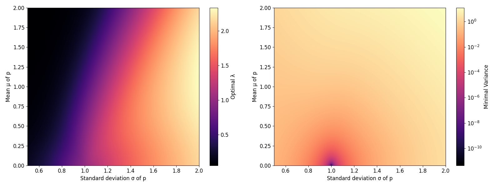
Interestingly, we see that when p has around the same mean and variance as q, the optimal choice of lambda is indeed given by around one. We can actually derive this analytically:

Derivation

Let \(L(x) = -\log r(x) + \lambda (r-1)\) be the estimator discussed before. Its variance is given by \(\mathrm{Var}_p[L(x)] = \mathrm{Var}_p[\log r(x)] + \lambda^2 \mathrm{Var}_p[r(x)] - 2 \lambda \mathrm{Cov}_p[\log r(x), r(x)]\)

To minimize this variance with respect to \(\lambda\), we take the derivative and set it to zero: \(\frac{d(\mathrm{Var})}{d\lambda} = 2 \lambda \mathrm{Var}_p[r(x)] - 2 \mathrm{Cov}_p[\log r(x), r(x)] = 0\)

Solving for \(\lambda\), we get the optimal value: \(\lambda_{opt} = \frac{\mathrm{Cov}_p[\log r(x), r(x)]}{\mathrm{Var}_p[r(x)]}\)

Massaging the expression for \(\mathrm{Cov}_p[\log r(x), r(x)]\) by again noting that \(E_p[r]=1\) and \(E_p[r-1]=0\), we obtain \(\begin{align} \mathrm{Cov}_p(\log r, r) &= E_p[(\log r - E_p[\log r])(r-1)] \\ &= E_p[(\log r)(r-1)] + E_p[\log r] E_p[r - 1]\\ &= E_p[(\log r)(r-1)] \end{align}\)

Which yields \(\lambda_{opt} = \frac{E_p[ \log r(x) (r(x) - 1) ]}{E_p[ (r(x) - 1)^2 ]}\)

Great! Now let’s do first handwavy approximation of \(\lambda_{opt}\) under the assumption that \(\epsilon(x) = r(x)-1\) is small. Indeed \(\log(1+\epsilon) = \epsilon + \mathcal O(\epsilon^2)\), so \(\lambda_{opt} = \frac{E_p[(\log (1+\epsilon(x))) \epsilon(x)]}{E_p[\epsilon(x)^2]} = \frac{E_p[(\epsilon(x) + \mathcal O(\epsilon(x)^2)) \epsilon(x)]}{E_p[\epsilon(x)^2]} \approx \frac{E_p[\epsilon(x)^2]}{E_p[\epsilon(x)^2]}= 1\)

As I will soon be receveing a degree in mathematics, I feel morally obliged to also include an explanation that is less likely to make a mathematician’s eyes bleed:

Same thing but more rigorous

Assume \(p_n\) and \(q_n\) are sequences of probability distributions such that the ratio \(r_n(x) = q_n(x)/p_n(x)\) has finite variance and converges uniformly to 1 as \(n \to \infty\). Then with \(\epsilon_n = r_n(x) -1\), we apply Cauchy-Schwarz to obtain that for \(n\) large enough,

Now since \(\epsilon_n\) goes to zero uniformly, \(\sup_{x\in \mathbb R} \epsilon_n(x)\) goes to zero, this proves that \(\lambda_{opt,n} \to 1\) as \(n \to \infty\)

Small note: division by zero is not a problem since the ratio \(r\) has variance one iff \(p=q\), in which case any \(\lambda\) results in zero variance. Note furthermore that we never explicitly needed the probability distributions to admit densitites - the entire proof also tracks with a Radon-Nikodym derivative that has finite variance and converges uniformly to one.

Important caveat: this rigorous proof does not yet prove that the optimal \(\lambda\) converges in the gaussian case we visualized above (because convergence of the ratio is not uniform)